Squeezing million-cell preprocessing into 5 GB: anndataoom's cascading lazy views

Single-cell atlases routinely cross a million cells, while the standard analysis stack reads the entire expression matrix into RAM — peak RAM grows linearly with cell count and quickly exhausts an ordinary workstation. anndataoom swaps in a different data representation to get around that wall: instead of treating the matrix as "an in-memory substrate that every step rewrites," it treats it as a stack of composable on-disk views to be read through. Here are the design trade-offs, and how it differs from existing approaches.

Single machine	Peak memory	Memory saved (same scale)	Million-cell full run
1,053,033 cells	~5.0 GB (constant)	≈53×	44.8 min

The problem: a million cells hit the memory wall

Mainstream AnnData keeps the cell × gene matrix as a dense or sparse array in RAM, and preprocessing (QC, normalization, log, HVG, scaling, PCA) repeatedly reads and rewrites that in-memory matrix. The model is simple and fast, but peak memory grows linearly with cell count: a 10⁶ cell × 6×10⁴ gene sparse count matrix is already tens of GB, and densifying transforms like scale / Pearson residuals / regression momentarily blow that up by another order of magnitude.

Existing out-of-core approaches each solve only half: disk-backed mode defers loading, but the moment a transform touches the data it reads the whole block into memory; general chunking frameworks (e.g. Dask) can stream a single operator, but the standard preprocessing functions are written against in-memory arrays and materialize anyway. What's really missing is keeping the entire multi-step pipeline — not just one step — lazy and chunked end to end.

One data point: on TS-Epi (228,032 cells), the sparse raw matrix is only ~11 GB on disk, yet the in-memory peak reaches 107 GB. The extra ~96 GB is dense intermediate product, not data.

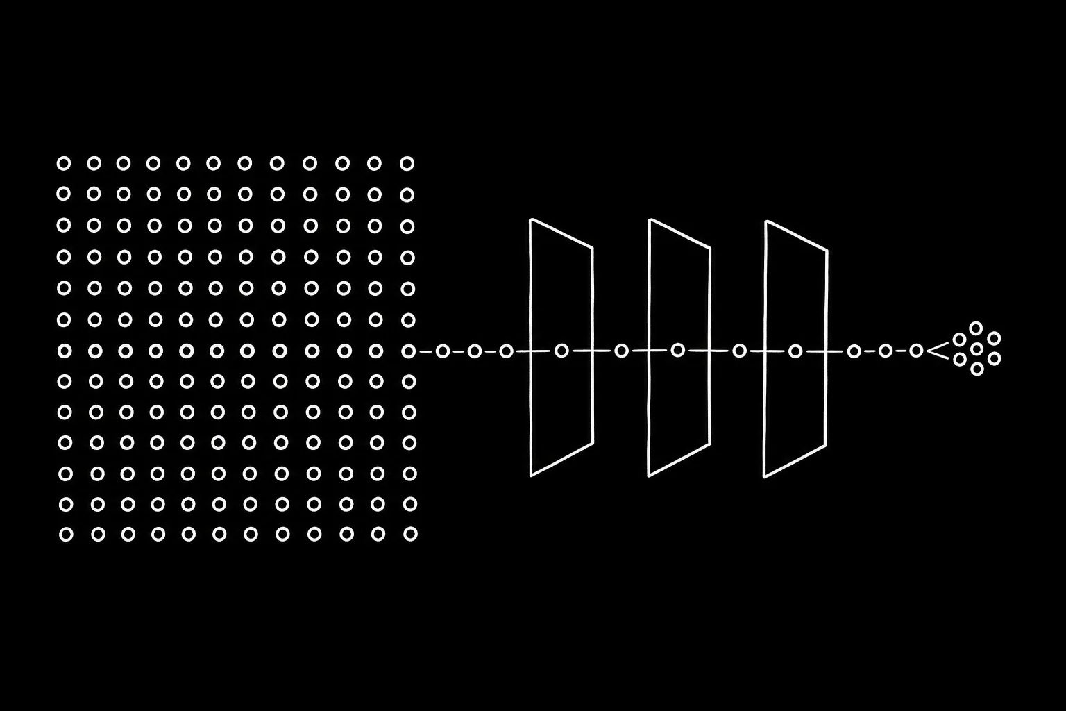
The core idea: don't rewrite the matrix — view it

Key observation: single-cell preprocessing is essentially a composition of "expensive to evaluate, tiny to describe" local maps. Normalization divides each row by a scalar; log1p is element-wise; scaling subtracts a per-gene mean and divides by std; Pearson residuals are a closed form of row and column sums; regression subtracts a per-gene least-squares fit over a small design matrix.

None of them needs "the whole matrix in memory" to be described — they only need O(cells)+O(genes) small vectors, and they're all local: each element's transformed value depends only on itself and those small parameters. The in-memory design ignores this structure, treating the matrix as both "storage" and "a substrate every step rewrites," so peak memory is pinned to the matrix itself.

The design principle: separate the "description of the transform" (tiny, composable) from the "evaluation of the transform" (per chunk, computed on read). Each step is a view that wraps its parent and computes the transform on each chunk at read time. An N-step pipeline thus collapses into a single streaming pass, with peak memory equal to one chunk, independent of cell count.

That dense "processed matrix" never actually exists (in full form): it's just intermediate waste. What downstream actually wants is small — the PCA coordinates n_obs×50, HVG flags, QC metrics. What anndataoom skips is exactly the one thing that grows linearly with cell count.

The cascading view hierarchy

The matrix is represented as a stack of array views, each exposing the same minimal interface (shape, chunked row iterator, row read), reading either raw bytes from disk or a transform applied to the chunk its parent yields. Higher-order transforms compose by calling the parent transform first (super()._transform_chunk) — the subclass hierarchy is the algebraic structure of the transforms. A real pipeline view chain looks like this:

X (HDF5 on disk, Rust I/O via anndata-rs)
  → TransformedBackedArray   normalize: ÷ per-cell size factor
    → TransformedBackedArray   log1p: on the fly
      → _SubsetBackedArray   HVG: select 2,000 gene columns (O(1))
        → ScaledBackedArray   z-score: stores only mean/std vectors
          → Randomized SVD   chunked matrix products
            → X_pca   n_obs × 50, in memory
              → Neighbors / UMAP / Leiden   operate on X_pca only

Each layer stores only O(cells) or O(genes) small parameters (mean/std for 2,000 genes is ~16 KB), and never writes out the full transformed matrix:

View layer	Wraps	State stored	Computed per chunk on read
BackedArray	disk (anndata-rs)	shape, file handle	none — raw slice read
TransformedBackedArray	BackedArray	per-cell divisor; log flag	x / factor; log1p(x)
_SubsetBackedArray	any view	row / column indices	O(1) subset (e.g. 2,000 HVG columns)
ScaledBackedArray	Transformed	per-gene mean, std; clip	(x − μ)/σ, clipped
PearsonResidualBackedArray	Transformed	row/column sums; θ, clip	(x − μ)/√(μ + μ²/θ)
RegressedBackedArray	Transformed	betas (k×n_vars); design matrix C	x − C·β

Three implementation details

Fusion + chain re-basing: commutative normalize+log1p fuse into a single layer; stacking a new transform on a view that is already a TransformedBackedArray re-bases onto its original parent and forwards the parent parameters. So chain depth stays ≤ 2, and "add a step = O(1) overhead" / "N steps collapse to one pass" hold literally.

Sparsity preserved by semantics: the view knows "division preserves zeros, log1p(0)=0," so normalize+log1p still yield sparse chunks; only the intrinsically dense scale/pearson/regress densify, and only one chunk at a time.

No numerical drift: each step computes from the original data, not stacked on already-rounded float32 intermediates; measured bit-level agreement with scanpy (normalize+log1p 2.4e-7, pearson 3.8e-6, regress 6e-7).

Why it's better than prior designs

Strategy	Peak memory	N-step read/write	Keeps sparse	Rewrite functions	Finishes 1M
in-memory (scanpy/ov)	O(cells×genes)×2–3	read 1×	only norm/log	no	no
backed mode	O(cells×genes) (transform = materialize)	1×	no	no	no
naive chunk-rewrite	O(chunk)	~2N× + N on-disk temp files	lost on first write	yes	yes (I/O-bound)
general lazy arrays (Dask/Zarr)	O(chunk)	~1×	engine-dependent	port every function	maybe
view cascade (anndataoom)	O(chunk)	read 1×, no scratch	norm/log throughout; rest 1 chunk dense	no (one-line dispatch)	yes

Versus the "most obvious" naive chunk-rewrite: it can also achieve O(chunk), but at the cost of a full read + full write per step (~2N× I/O) + N on-disk temp files, and once it writes a dense intermediate it loses sparsity. The view cascade saves all of that with "fuse + read once + don't land." And versus Dask/general lazy arrays: they don't know the domain facts (log1p preserves zeros, normalize commutes, only HVG needs densifying), and you'd have to port the whole function suite to a new array type; the view cascade is domain-specific, so zero rewrite, sparsity preserved.

Performance: from 5k to a million cells

Running the standard pipeline on the Tabula Sapiens series (5,000 → 1,053,033 cells, all 60,606 genes) under a 256 GB memory cap. The memory of in-memory and scanpy-backed grows linearly with cell count and gets OOM-killed past ~230k cells; anndataoom's peak stays essentially constant (0.9 → 5.2 GB) and is the only configuration that finishes a million cells.

Constant memory costs no speed: past the smallest dataset, anndataoom sits in the same time band as in-memory, and is even faster on TS-Epi (800.7 s vs 880.1 s); the full million-cell run is 44.8 min (2,688.7 s). Only on TS-5k — where the dense matrix fits easily — does the fixed overhead of chunked iteration show, and that case doesn't need out-of-core anyway.

CPU and CPU–GPU mixed backends are largely time-insensitive (TS-1M: 2,811 s vs 2,689 s, same ~5 GB) — out-of-core pipelines are mostly bounded by I/O and chunk scheduling, not raw compute.

One set of operators, two backing stores

The same idea can also slim down in-memory: a view's backing is just "an array-like that can yield chunks," so the same chunked operators + implicit-centering PCA are agnostic to whether the matrix lives on disk or in RAM. Applied to an in-memory sparse matrix, it kills in-memory's main blow-ups — the transient dense copies in scale/pearson/PCA — without changing the original sparse O(nnz) footprint.

Our implicit-centering configuration is exactly this idea applied to PCA: TS-Epi peak drops from ~107 GB to ~48 GB, and it even runs the 592k that dense PCA can't. But we deliberately stop there — we don't lazify the whole in-memory matrix: anndataoom already covers the "doesn't fit" case, eager dense kernels are faster when it does fit, and full lazification would break the ecosystem's concrete-array assumptions and slow the fast path. In one line: one set of operators, two backing stores (RAM for a slimmer in-memory, disk for constant-memory out-of-core).

Getting started: three lines to read, lazy throughout

pip install anndataoom

Prebuilt wheels bundle a static HDF5 — no system dependencies, no Rust toolchain (Linux x86_64 / macOS arm64·x86_64 / Windows x86_64 (0.1.8+), Python 3.10–3.12). Usage is transparent: read with anndataoom, then call ov.pp.* as usual, and the whole qc → preprocess → HVG subset → scale → PCA → neighbors/UMAP/Leiden runs out-of-core without changing a line of call code; ov.pl.* plotting (including use_raw=True) works as usual too.

import anndataoom as oom, omicverse as ov

adata = oom.read("atlas_1M.h5ad")          # matrix stays on disk, X is a lazy BackedArray
ov.pp.qc(adata, doublets=False)            # QC: one chunked scan, writes only obs/var
ov.pp.preprocess(adata, mode="shiftlog|pearson", n_HVGs=2000)
adata.raw = adata
adata = adata[:, adata.var.highly_variable_features]  # O(1) lazy column subset
ov.pp.scale(adata)                         # lazy z-score (stores only mean/std vectors)
ov.pp.pca(adata, layer="scaled", n_pcs=50) # chunked randomized SVD
ov.pp.neighbors(adata, n_pcs=50); ov.pp.umap(adata); ov.pp.leiden(adata)
ov.pl.embedding(adata, basis="X_umap", color="leiden")  # peak ≈ one chunk throughout

The standard preprocessing surface is covered: qc, normalize_total, log1p, highly_variable_genes, scale, pca, filter_cells/genes, normalize_pearson_residuals, regress all take the OOM path; scrublet takes a bounded "materialize only the HVG subset" path. Unsupported sub-cases raise a clear exception at the call site — never silently miscompute.

Limitations and notes

• PCA accuracy: by default it runs a single in-memory randomized SVD (sklearn) on the HVG submatrix, highly consistent with standard PCA for the top ~50 PCs common in single-cell (the spectrum decays fast; measured |cos| = 1.0); only synthetic / strongly-batched data with a slow-decaying spectrum needs more power iterations.
• Writing back to X is lazy: adata[mask] = value triggers a materialize; to persist changes use adata.write(path) (chunked write, no materialize) or modify obs/obsm.
• A few intrinsically-global operators (some non-Harmony batch correction, etc.) still need a materialize and run with a warning.
• File locks: default backed='r' is read-only and protects the source file; HDF5 takes an exclusive lock by default, so reading the same file from multiple processes needs HDF5_USE_FILE_LOCKING=FALSE.

Closing

With the right data representation, million-cell single-cell preprocessing can run at constant memory: represent the pipeline as a stack of composable on-disk views, collapse it into a single lazy pass, keep sparsity where the math allows, and expose it under unchanged API names. In other words, constant memory is a property of the representation itself, not an optimization bolted on afterward — what looked like a memory-engineering problem becomes, with the right representation, a data-representation problem.

It builds on scverse/anndata-rs (a Rust implementation of AnnData, © Kai Zhang), pinned to a fixed commit for reproducibility (same lineage as SnapATAC2). MIT license.

@software{anndataoom,
  title  = {anndata-oom: out-of-memory AnnData for constant-memory
            single-cell preprocessing},
  author = {Zeng, Zehua and {the anndata-oom contributors}},
  url    = {https://github.com/omicverse/anndata-oom},
  year   = {2026},
}